← Back to Tutorials Chapter 6: Supervised Learning

Supervised Learning in Depth

Supervised learning is the most common ML paradigm. It involves learning a function that maps inputs to outputs based on labeled training data. This chapter covers regression, classification, and the most popular supervised algorithms.

Regression vs Classification

Regression predicts continuous values (e.g., house price, temperature). Classification predicts discrete class labels (e.g., spam vs not spam, digit recognition). Evaluation metrics differ: regression uses MSE, MAE, R-squared; classification uses accuracy, precision, recall, F1-score.

Linear Regression

Linear regression models the relationship between input features and a continuous target using a linear equation. It is simple, interpretable, and serves as a baseline for more complex models.

from sklearn.linear_model import LinearRegression
from sklearn.metrics import mean_squared_error

model = LinearRegression()
model.fit(X_train, y_train)
y_pred = model.predict(X_test)

mse = mean_squared_error(y_test, y_pred)
print(f"MSE: {mse:.2f}")

Decision Trees

Decision trees split data based on feature values, forming a tree structure. They are intuitive and handle both numerical and categorical data. However, they tend to overfit without proper pruning or depth limits.

from sklearn.tree import DecisionTreeClassifier

tree = DecisionTreeClassifier(max_depth=5, random_state=42)
tree.fit(X_train, y_train)
accuracy = tree.score(X_test, y_test)
print(f"Accuracy: {accuracy:.2f}")

Random Forest

Random forest builds many decision trees and averages their predictions. It reduces overfitting, handles high-dimensional data, and provides feature importance scores. It is one of the most robust off-the-shelf algorithms.

Support Vector Machines (SVM)

SVM finds the hyperplane that best separates classes. It works well for high-dimensional spaces and uses kernel tricks to handle non-linear boundaries. Common kernels include linear, polynomial, and RBF.

K-Nearest Neighbors (KNN)

KNN predicts based on the majority class or average value of the k closest training examples. It is non-parametric and simple but becomes slow with large datasets. Feature scaling is critical for KNN.

from sklearn.neighbors import KNeighborsClassifier

knn = KNeighborsClassifier(n_neighbors=5)
knn.fit(X_train, y_train)
y_pred = knn.predict(X_test)

Train/Evaluate Pipeline

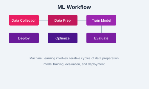
A typical supervised learning pipeline: load data, split, preprocess, train, evaluate, tune hyperparameters, and validate. Use cross-validation for more reliable performance estimates.

from sklearn.model_selection import cross_val_score

scores = cross_val_score(model, X, y, cv=5)
print(f"CV accuracy: {scores.mean():.2f} (+/- {scores.std() * 2:.2f})")

Model Selection

Choosing the right model involves trade-offs. Consider bias-variance tradeoff, interpretability, training time, prediction time, and data size. Try multiple models and compare their cross-validation scores.

Note: Always start with a simple baseline (e.g., linear regression for regression, logistic regression for classification) before trying complex models.

Summary

Supervised learning offers powerful tools for prediction. Master linear regression, decision trees, random forest, SVM, and KNN. Practice building end-to-end pipelines with proper evaluation.

Exercise 6.1: Load the Boston housing dataset (or California housing). Train a linear regression, decision tree, and random forest model. Compare their MSE and R-squared scores. Use cross-validation and discuss which model performed best and why.